How to Edit Pivot Table in Excel: A Complete Step-by-Step Guide

Microsoft Excel is one of the most popular tools for organising, analysing, and managing data. It offers many useful features that make working with large datasets easier. One of these features is the PivotTable, which helps users summarise information, compare values, and understand data quickly.

However, many beginners find it difficult to make changes to an existing PivotTable. They may want to add new columns, change calculations, update data, or rearrange information.

If you are wondering how to edit pivot table in Excel, you are in the right place. This guide explains everything in simple steps, from changing PivotTable fields to updating source data and modifying its layout.

Whether you are a student, office worker, business owner, or Excel beginner, these instructions will help you manage your PivotTables more easily.

What Is a PivotTable in Excel?

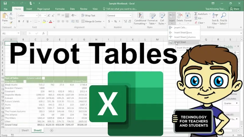
A PivotTable is an Excel feature that allows users to summarise and analyse large amounts of information without manually calculating every value.

For example, imagine you have a sales spreadsheet containing hundreds of records. It includes product names, sales dates, employee names, and prices.

Instead of reviewing every row, you can create a PivotTable to find:

• Total sales for each product.
• Monthly sales performance.
• Sales made by individual employees.
• Average order values.
• Highest and lowest sales amounts.

PivotTables organise information into a simple format, making it easier to understand important details.

How to Edit Pivot Table in Excel

Editing a PivotTable is simple once you understand where its main options are located.

Follow these steps to make changes to an existing PivotTable.

Step 1: Open Your Excel File

First, open Microsoft Excel on your computer.

Find the workbook containing the PivotTable you want to edit.

If you have not created a PivotTable yet, select your data and go to Insert, then choose PivotTable.

Step 2: Select the PivotTable

Click any cell inside your existing PivotTable.

After selecting it, Excel displays the PivotTable-related options in the ribbon.

Depending on your Excel version, you may see tabs such as:

• PivotTable Analyze
• Design

These tabs contain the tools you need to modify your PivotTable.

Step 3: Open the PivotTable Field List

The Field List allows you to control which information appears in your PivotTable.

To open it:

1. Click anywhere inside the PivotTable.
2. Open the PivotTable Analyze tab.
3. Select Field List.
4. Wait for the field panel to appear.

You will see the available columns from your original dataset.

The Field List usually contains four main areas:

Filters: Add filters to control which records appear in the report.

Columns: Display selected information across columns.

Rows: Display information vertically in rows.

Values: Show calculations such as sums, counts, and averages.

Step 4: Add or Remove Fields

You can change the information displayed in your PivotTable by moving fields between different areas.

For example, if your PivotTable displays total sales by product, you can add an employee field to see which employees generated those sales.

To add a field:

1. Find the required field in the Field List.
2. Drag it into the Rows, Columns, Values, or Filters area.
3. Check the updated PivotTable.

To remove a field, drag it outside the four areas or uncheck its name.

This is one of the easiest ways to customise an existing PivotTable.

How to Change Values in a PivotTable

Sometimes you may want to change how Excel calculates the information in your PivotTable.

For example, instead of showing total sales, you may want to display average sales.

Follow these steps:

1. Click any number inside the Values area of your PivotTable.
2. Right-click and select Summarize Values By.
3. Choose the calculation you need.

Common calculation options include:

• Sum
• Count
• Average
• Maximum
• Minimum
• Product

You can also open Value Field Settings to access additional calculation and display options.

For example, selecting Average will show the average value instead of the total.

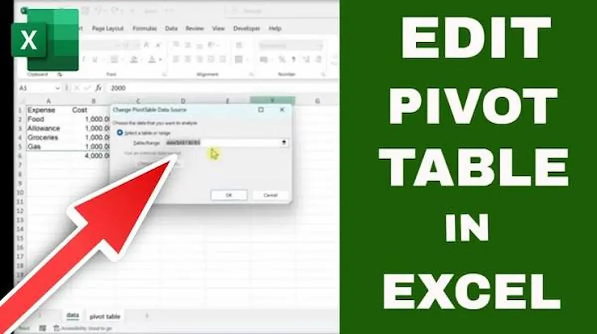
How to Change the Source Data of a PivotTable

If you have added new rows or columns to your original Excel dataset, you may need to update the PivotTable’s source data.

Here is how to do it:

1. Select any cell inside your PivotTable.
2. Open the PivotTable Analyze tab.
3. Click Change Data Source.
4. Select Change Data Source again if required.
5. Choose the updated data range.
6. Click OK.

Your PivotTable will now use the selected source range when refreshed.

Tip: Converting your original dataset into an Excel Table using Ctrl + T can make it easier to include new rows in future PivotTable updates.

How to Refresh a PivotTable in Excel

If you have changed information in your original dataset, the PivotTable may continue showing old results.

You need to refresh it to display the latest information.

Follow these steps:

1. Click anywhere inside your PivotTable.
2. Open the PivotTable Analyze tab.
3. Select Refresh.
4. Wait for Excel to update the results.

You can also right-click inside the PivotTable and select Refresh.

If you have multiple PivotTables in the same workbook, use Refresh All from the Data tab to update their connected data.

Remember that refreshing updates the PivotTable using its existing source range. If new rows are outside that range, you may need to change the data source first.

You may also like it:

How To Edit Image Text In Word – Aarya Editz 

How To Edit Video In Iphone – Aarya Editz 

How To Edit Resume In Laptop – Aarya Editz 

How To Edit Photos In Mobile – Aarya Editz

How to Change the Layout of a PivotTable

Excel allows you to change the appearance and structure of your PivotTable.

For example, you can display information in a compact, outline, or tabular format.

Follow these instructions:

1. Select your PivotTable.
2. Open the Design tab.
3. Click Report Layout.
4. Choose your preferred layout.

The available options include:

Compact Form: Displays multiple row fields in a compact structure.

Outline Form: Shows row fields in a more organised outline layout.

Tabular Form: Displays each row field in a separate column.

You can choose the format that makes your report easier to read.

How to Change the Formatting of a PivotTable

Formatting helps make your PivotTable more professional and understandable.

You can change its colours, fonts, borders, and number formats.

Here is how:

1. Select the PivotTable.
2. Open the Design tab.
3. Explore the PivotTable Styles section.
4. Select a style you like.
5. Adjust other formatting options if needed.

You can also change number formatting.

For example, if your PivotTable displays sales amounts, you can format the values as currency.

To do this:

1. Right-click a value in the PivotTable.
2. Select Value Field Settings.
3. Click Number Format.
4. Choose Currency, Percentage, Number, or another format.
5. Click OK.

This helps keep your data organised and easy to understand.

How to Filter Data in a PivotTable

Filters allow you to display only the information you want to analyse.

For example, you may want to see sales from a particular month or a specific product.

Follow these steps:

1. Select your PivotTable.
2. Find the field you want to filter.
3. Click its drop-down arrow.
4. Select or deselect the required items.
5. Click OK.

You can also use slicers to filter PivotTable information through interactive buttons.

To add a slicer:

1. Select the PivotTable.
2. Open PivotTable Analyze.
3. Click Insert Slicer.
4. Select the field you want to use.
5. Click OK.

A slicer will appear on your worksheet. You can click its buttons to filter the report.

How to Edit a PivotTable Without Changing Source Data

One important thing to understand is that PivotTables are connected to their original datasets.

You can change the way information is displayed without modifying the original data.

For example, you can:

• Move fields between rows and columns.
• Add or remove filters.
• Change calculations.
• Apply different layouts.
• Update number formatting.

However, if you want to change an original product name, sales amount, or employee record, you should edit the source data and refresh the PivotTable.

Directly typing over a calculated PivotTable value generally does not work because Excel controls those summary cells.

How to Edit Pivot Table in Excel on Mac

Mac users can also edit PivotTables in Microsoft Excel.

The process is similar to the Windows version.

1. Open your Excel workbook.
2. Select any cell inside the PivotTable.
3. Open the PivotTable Analyze tab.
4. Find the Field List option.
5. Add or remove fields as required.
6. Change calculations and formatting.
7. Refresh the PivotTable after updating the source data.

Some menu names and locations may differ slightly depending on your Excel version.

Common Problems When Editing PivotTables

Sometimes users experience problems while making changes to PivotTables. Here are some common issues and their solutions.

1. PivotTable Is Not Updating

This usually happens when the original dataset has changed but the PivotTable has not been refreshed.

Solution: Select the PivotTable and click Refresh. If you added new rows outside the source range, update the data source as well.

2. Field List Is Missing

Sometimes the Field List disappears from the worksheet.

Solution: Click inside the PivotTable, open PivotTable Analyze, and select Field List.

3. Cannot Edit PivotTable Cells

PivotTable summary cells are controlled by Excel, so you generally cannot type directly into them.

Solution: Change the source data or modify the fields and calculations through the PivotTable options.

4. New Data Is Not Appearing

This can happen when newly added records are outside the original source range.

Solution: Open Change Data Source, select the complete dataset, and refresh the PivotTable.

5. Wrong Calculation Is Showing

Your PivotTable may display Count instead of Sum or another calculation.

Solution: Open Value Field Settings and select the correct calculation option.

Tips for Managing PivotTables in Excel

Here are some useful tips to make working with PivotTables easier:

• Keep your original dataset organised.
• Use clear column headings.
• Avoid blank rows and columns in your source data.
• Convert source data into an Excel Table.
• Refresh PivotTables after changing source information.
• Use meaningful names for your fields.
• Apply number formatting to improve readability.
• Use filters and slicers to analyse specific information.
• Keep a backup of important Excel workbooks.

These practices can help you avoid common errors and manage large datasets more efficiently.

Frequently Asked Questions (FAQs)

Conclusion

Learning how to edit pivot table in Excel can make data management much easier. PivotTables allow you to organise information, change calculations, apply filters, and create useful reports without manually processing every record.

You can edit an existing PivotTable by using the Field List, changing its source data, updating calculations, and adjusting its layout. If you make changes to the original dataset, remember to refresh your PivotTable to display the latest results.

With regular practice, you can use Excel PivotTables to analyse information more efficiently and create clear, professional reports.